Lattice Boltzmann Method (LBM) - Basics
At mesoscopic level, fluid flows can be described by the Boltzmann equation $\frac{\partial f}{\partial t}+\xi \cdot \nabla f +\mathbf{F}\cdot \nabla_{\xi}f= \Omega$ based on gas kinetic theory. However, the computational cost would be extremely high if we try to resolve the length and time scales that are applicable to Boltzmann equation in practical engineering problems. On the other hand, in the lattice Boltzmann (LB) method, the evoluation equation of distribution function $f_{i}$ is written as $f_{i}(\mathbf{x}+\mathbf{e}_{i}\delta_{t}, t+\delta_{t})-f_{i}(\mathbf{x},t)=-\frac{1}{\tau}\left[ f_{i}(\mathbf{x},t)-f_{i}^{(\text{eq})}(\mathbf{x},t) \right]$, where $\tau$ is the relaxation time. Then, macroscopic fluid variables, such as density and velocity can be calculated as $\rho=\sum_{i} f_{i}$, $\mathbf{u}=\frac{1}{\rho}\sum_{i}\mathbf{e}_{i}f_{i}$.
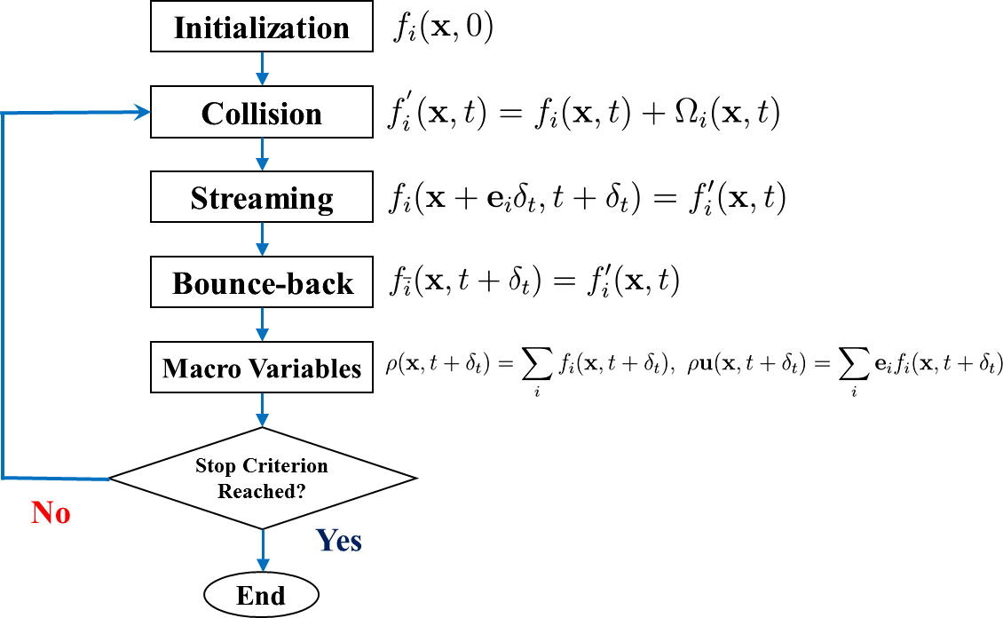
The standard implementation consists of four subroutines: collision, streaming, bounce-back, and calculating macro variables.
The advantages of the LB method (compared with convectional numerical methods based on solving Navier-Stokes equations) are:
- It is based on kinetic theory and is suitable for simulating complex flows (such as gas-liquid two-phase flows, particulate flows, and flows in porous media).
- It is not necessary to solve Poisson equation for the pressure field.
- It is easy to be parallelized.